Data Analytics, we often use Model Development to help us predict future observations from the data we have.
-Linear Regression (선형 회귀): Simple Linear Regression is a method to help us understand the relationship between two variables:
The predictor/independent variable (X)
The response/dependent variable (that we want to predict)(Y)
The result of Linear Regression is a linear function that predicts the response (dependent) variable as a function of the predictor (independent) variable.
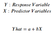
- a refers to the intercept of the regression line0, in other words: the value of Y when X is 0
- b refers to the slope of the regression line, in other words: the value with which Y changes when X increases by 1 unit
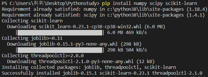
우선 Liner Regression을 파이썬에서 사용하기 위해서는 프롬프트 창에서 install을 해야한다.
pip install numpy scipy scikit-learn
예) Y= ax +b 일시 'a' 값 과 'b'값 구하기
import pandas as pd
import numpy as np
import matplotlib.pyplot as plt

path = 'https://s3-api.us-geo.objectstorage.softlayer.net/cf-courses-data/CognitiveClass/DA0101EN/automobileEDA.csv'
df = pd.read_csv(path)
# print(df.head())

from sklearn.linear_model import LinearRegression

#Create the linear regression object
lm = LinearRegression()
# print(lm)


X = df[['highway-mpg']]
Y = df['price']
print(lm.fit(X,Y))
Yhat=lm.predict(X)

#We can output a prediction
print(Yhat[0:5])

print('intercept value:', lm.intercept_)
print('coef value:', lm.coef_)
>>
LinearRegression()
[16236.50464347 16236.50464347 17058.23802179 13771.3045085
20345.17153508]
intercept value: 38423.305858157386
coef value: [-821.73337832]
최종공식: price = 38423.31 - 821.73 x highway-mpg
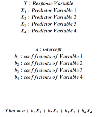
- Multiple Linear Regression (다중 선형 회귀): 2개 이상의 variable의 영향을
What if we want to predict car price using more than one variable?
If we want to use more variables in our model to predict car price, we can use Multiple Linear Regression. Multiple Linear Regression is very similar to Simple Linear Regression, but this method is used to explain the relationship between one continuous response (dependent) variable and two or more predictor (independent) variables. Most of the real-world regression models involve multiple predictors. We will illustrate the structure by using four predictor variables, but these results can generalize to any integer:
예) 다중선형회귀 공식 도출하기
import pandas as pd
import numpy as np
import matplotlib.pyplot as plt

path = 'https://s3-api.us-geo.objectstorage.softlayer.net/cf-courses-data/CognitiveClass/DA0101EN/automobileEDA.csv'
df = pd.read_csv(path)
# print(df.head())

from sklearn.linear_model import LinearRegression

#Create the linear regression object
lm = LinearRegression()

Z = df[['horsepower', 'curb-weight', 'engine-size', 'highway-mpg']]
print(lm.fit(Z, df['price']))
print('intercept value:', lm.intercept_)
print('coef value:', lm.coef_)
>>
LinearRegression()
intercept value: -15806.624626329227
coef value: [53.49574423 4.70770099 81.53026382 36.05748882]
𝑌ℎ𝑎𝑡=𝑎+𝑏1𝑋1+𝑏2𝑋2+𝑏3𝑋3+𝑏4𝑋4
Price = -15678.742628061467 + 52.65851272 x horsepower + 4.69878948 x curb-weight + 81.95906216 x engine-size + 33.58258185 x highway-mpg
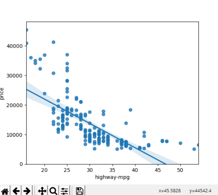
예) Graph 그리기
import seaborn as sns
sns.regplot(x="highway-mpg", y="price", data=df)
plt.ylim(0,)
plt.show()
>>
'IT > Python' 카테고리의 다른 글
| [파이썬] Pandas Cheat Sheet (0) | 2020.06.17 |
|---|---|
| [파이썬] Model Development (Residual Plot) (0) | 2020.06.16 |
| [파이썬] Data Analysis (0) | 2020.06.13 |
| [파이썬] Data wrangling (0) | 2020.06.12 |
| [파이썬] Model Evaluation using Visualization (Model Development) (0) | 2020.06.12 |


